# The Complete Pure & Applied Mathematics Roadmap

The Complete Pure & Applied Mathematics Roadmap

A stage-by-stage study guide with concepts, formulas, prerequisites, and learning order

How to read this guide: Mathematics is a dependency graph, not a list. Each stage below unlocks the next. Skipping ahead is the single most common reason people stall. Work top-to-bottom, and only branch into Pure vs. Applied after Stage 1 is solid.

One of your stored documents — _OceanofPDF.com_Finite_Math_For_Dummies_-_Mary_Jane_Sterling — maps almost perfectly onto the Finite / Discrete-Applied module in Stage 1B and the Operations Research track in Stage 3. I've woven its exact topics and formulas into the relevant sections and flagged them with 📘.

1. The Dependency Map

text

                    ┌─────────────────────────────┐
                    │  STAGE 0: FOUNDATIONS       │
                    │  Algebra · Geometry · Trig  │
                    │  Functions · Precalculus    │
                    └──────────────┬──────────────┘
                                   │
                    ┌──────────────▼──────────────┐
                    │  STAGE 1: THE CORE TRUNK    │
                    │  Calculus I–III             │
                    │  Linear Algebra             │
                    │  Proofs & Discrete Math 📘  │
                    │  Ordinary Diff. Equations   │
                    └───────┬─────────────┬───────┘
                            │             │
         ┌──────────────────▼──┐       ┌──▼────────────────────┐
         │  STAGE 2: PURE      │       │  STAGE 3: APPLIED     │
         │  Real Analysis      │◄─────►│  Probability & Stats  │
         │  Abstract Algebra   │       │  Numerical Analysis   │
         │  Topology           │       │  PDEs & Fourier       │
         │  Complex Analysis   │       │  Optimization / LP 📘 │
         │  Number Theory      │       │  Dynamical Systems    │
         │  Measure Theory     │       │  OR & Game Theory 📘  │
         │  Functional Anal.   │       │  Financial Math 📘    │
         │  Diff. Geometry     │       │  Info Theory / ML     │
         │  Algebraic Topology │       │  Math Modeling        │
         └─────────────────────┘       └───────────────────────┘
                            │             │
                    ┌───────▼─────────────▼───────┐
                    │  STAGE 4: RESEARCH FRONTIER │
                    └─────────────────────────────┘

A real university prerequisite chart for the applied side (University of Arizona) looks like this:

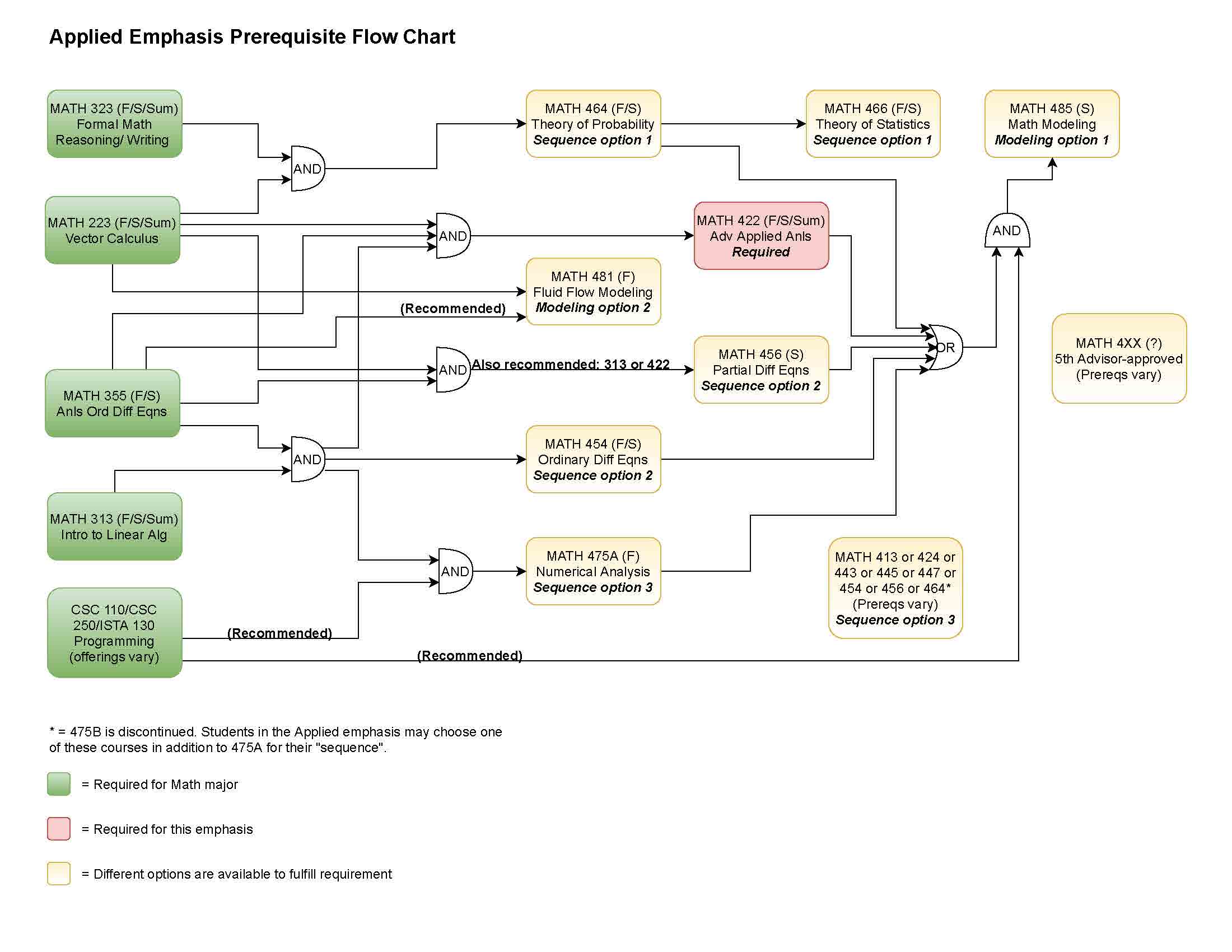$Applied Mathematics prerequisite flow chart$ Source: University of Arizona Math Center prerequisite flow charts

2. STAGE 0 — Foundations (Prerequisite Layer)

Goal: total fluency in symbol manipulation. You should never have to think about these — they must be automatic.

2.1 Topic Checklist

Number systems: ℕ ⊂ ℤ ⊂ ℚ ⊂ ℝ ⊂ ℂ
Exponents, radicals, logarithms
Polynomial & rational expressions, factoring, partial fractions
Equations & inequalities (linear, quadratic, absolute value, rational)
Functions: domain, range, composition, inverses, transformations
Analytic geometry: lines, circles, conics
Trigonometry: unit circle, identities, equations, laws
Sequences, series, binomial theorem
Complex numbers & polar form

2.2 Formula Sheet — Algebra

Concept	Formula
Exponent laws	aᵐ·aⁿ = aᵐ⁺ⁿ ; (aᵐ)ⁿ = aᵐⁿ ; a⁻ⁿ = 1/aⁿ ; a^(1/n) = ⁿ√a
Log laws	log(xy) = log x + log y ; log(x/y) = log x − log y ; log(xⁿ) = n log x
Change of base	log_b x = ln x / ln b
Quadratic formula	x = (−b ± √(b² − 4ac)) / 2a ; discriminant Δ = b² − 4ac
Vieta's formulas	x₁ + x₂ = −b/a ; x₁x₂ = c/a
Difference of squares	a² − b² = (a − b)(a + b)
Sum/diff of cubes	a³ ± b³ = (a ± b)(a² ∓ ab + b²)
Binomial theorem	(a + b)ⁿ = Σ_{k=0}^{n} C(n,k) aⁿ⁻ᵏ bᵏ
Arithmetic series	aₙ = a₁ + (n−1)d ; Sₙ = n(a₁ + aₙ)/2
Geometric series	aₙ = a₁rⁿ⁻¹ ; Sₙ = a₁(1 − rⁿ)/(1 − r) ; S∞ = a₁/(1 − r), \|r\| < 1

2.3 Formula Sheet — Geometry & Analytic Geometry

Concept	Formula
Distance	d = √((x₂ − x₁)² + (y₂ − y₁)²)
Midpoint	M = ((x₁ + x₂)/2, (y₁ + y₂)/2)
Slope 📘	m = (y₂ − y₁)/(x₂ − x₁) = Δy/Δx
Slope-intercept form 📘	y = mx + b
Point-slope form 📘	y − y₁ = m(x − x₁)
Standard form 📘	Ax + By = C → slope = −A/B, y-int = C/B, x-int = C/A
Parallel / perpendicular 📘	m₁ = m₂ / m₁·m₂ = −1
Circle	(x − h)² + (y − k)² = r²
Ellipse	(x−h)²/a² + (y−k)²/b² = 1
Hyperbola	(x−h)²/a² − (y−k)²/b² = 1
Parabola	(x − h)² = 4p(y − k)

📘 The line-equation block above is exactly Chapter 2 of your Finite Math text — "Recognizing Equations of Lines," including converting between slope-intercept and standard form, horizontal/vertical lines, and lines through the origin (_OceanofPDF.com_Finite_Math_For_Dummies_-_Mary_Jane_Sterling, pp. 19–32).

2.4 Formula Sheet — Trigonometry

Concept	Formula
Pythagorean	sin²θ + cos²θ = 1 ; 1 + tan²θ = sec²θ ; 1 + cot²θ = csc²θ
Sum/difference	sin(A±B) = sinA cosB ± cosA sinB ; cos(A±B) = cosA cosB ∓ sinA sinB
Double angle	sin2θ = 2 sinθ cosθ ; cos2θ = cos²θ − sin²θ = 2cos²θ − 1 = 1 − 2sin²θ
Half angle	sin²θ = (1 − cos2θ)/2 ; cos²θ = (1 + cos2θ)/2
Law of sines	a/sinA = b/sinB = c/sinC = 2R
Law of cosines	c² = a² + b² − 2ab cosC
Euler's formula	e^{iθ} = cosθ + i sinθ
De Moivre	(cosθ + i sinθ)ⁿ = cos nθ + i sin nθ

3. STAGE 1 — The Core Trunk

This is the non-negotiable shared foundation for both branches. Budget 12–24 months.

3.1 Calculus I — Differential Calculus

Concepts: limits, continuity, the derivative as a limit and as a rate of change, differentiation rules, implicit differentiation, related rates, extrema & optimization, curve sketching, Mean Value Theorem, linear approximation.

Concept	Formula
Derivative definition	f′(x) = lim_{h→0} [f(x+h) − f(x)]/h
Power rule	d/dx(xⁿ) = n·xⁿ⁻¹
Product rule	(uv)′ = u′v + uv′
Quotient rule	(u/v)′ = (u′v − uv′)/v²
Chain rule	d/dx f(g(x)) = f′(g(x))·g′(x)
Exponential / log	d/dx eˣ = eˣ ; d/dx aˣ = aˣ ln a ; d/dx ln x = 1/x
Trig	(sin x)′ = cos x ; (cos x)′ = −sin x ; (tan x)′ = sec²x
Inverse trig	(arcsin x)′ = 1/√(1 − x²) ; (arctan x)′ = 1/(1 + x²)
Mean Value Theorem	f′(c) = [f(b) − f(a)]/(b − a)
L'Hôpital's rule	lim f/g = lim f′/g′ for 0/0 or ∞/∞
Linearization	L(x) = f(a) + f′(a)(x − a)
Newton's method	xₙ₊₁ = xₙ − f(xₙ)/f′(xₙ)

3.2 Calculus II — Integral Calculus & Series

Concepts: antiderivatives, FTC, integration techniques, improper integrals, applications (area, volume, arc length, work), infinite sequences and series, power/Taylor series, polar & parametric curves.

Concept	Formula
FTC (Part 1 & 2)	d/dx ∫ₐˣ f(t)dt = f(x) ; ∫ₐᵇ f = F(b) − F(a)
Power rule	∫xⁿ dx = xⁿ⁺¹/(n+1) + C, n ≠ −1
Integration by parts	∫u dv = uv − ∫v du
Trig substitution	√(a²−x²)→x=a sinθ ; √(a²+x²)→x=a tanθ ; √(x²−a²)→x=a secθ
Disk / washer volume	V = π∫[R(x)² − r(x)²] dx
Shell volume	V = 2π∫ x·f(x) dx
Arc length	L = ∫√(1 + (f′(x))²) dx
Surface of revolution	S = 2π∫ f(x)√(1 + (f′(x))²) dx
Geometric series	Σ arⁿ = a/(1 − r), \|r\| < 1
p-series	Σ 1/nᵖ converges ⟺ p > 1
Ratio test	L = lim \|aₙ₊₁/aₙ\| ; converges if L < 1
Taylor series	f(x) = Σ f⁽ⁿ⁾(a)(x − a)ⁿ / n!
Key expansions	eˣ = Σxⁿ/n! ; sin x = Σ(−1)ⁿx²ⁿ⁺¹/(2n+1)! ; 1/(1−x) = Σxⁿ

3.3 Calculus III — Multivariable & Vector Calculus

Concept	Formula
Gradient	∇f = ⟨f_x, f_y, f_z⟩
Directional derivative	D_u f = ∇f · û
Multivariable chain rule	dz/dt = (∂z/∂x)(dx/dt) + (∂z/∂y)(dy/dt)
Second derivative test	D = f_xx f_yy − (f_xy)² ; D>0 & f_xx>0 → min
Lagrange multipliers	∇f = λ∇g subject to g = c
Jacobian	dA = \|∂(x,y)/∂(u,v)\| du dv
Line integral	∫_C F · dr = ∫ F(r(t))·r′(t) dt
Green's theorem	∮_C P dx + Q dy = ∬_R (Q_x − P_y) dA
Stokes' theorem	∮_C F·dr = ∬_S (∇×F)·dS
Divergence theorem	∯_S F·dS = ∭_V (∇·F) dV

3.4 Linear Algebra 📘

Concepts: systems of equations, matrices, determinants, vector spaces, linear independence, basis & dimension, linear transformations, eigen-theory, inner products, orthogonality, decompositions.

Concept	Formula
Matrix multiplication 📘	(AB)ᵢⱼ = Σₖ aᵢₖ bₖⱼ — not commutative
Transpose 📘	(Aᵀ)ᵢⱼ = aⱼᵢ ; (AB)ᵀ = BᵀAᵀ
2×2 determinant	det = ad − bc
2×2 inverse 📘	A⁻¹ = (1/(ad − bc))·[[d, −b], [−c, a]]
Inverse property 📘	AA⁻¹ = A⁻¹A = I
Cramer's rule	xᵢ = det(Aᵢ)/det(A)
Rank–nullity	rank(A) + nullity(A) = n
Eigen equation	Av = λv ; det(A − λI) = 0
Diagonalization	A = PDP⁻¹ ; Aᵏ = PDᵏP⁻¹
Trace / determinant	tr(A) = Σλᵢ ; det(A) = Πλᵢ
Projection	proj_u v = (v·u/u·u)u
Gram–Schmidt	uₖ = vₖ − Σ proj_{uᵢ} vₖ
SVD	A = UΣVᵀ
Norms	‖v‖₂ = √(Σvᵢ²) ; Cauchy–Schwarz: \|u·v\| ≤ ‖u‖‖v‖

📘 Your stored text covers the computational half of this beautifully: matrix dimension, identity matrices, addition/subtraction, scalar multiplication, transposes, row operations, row-echelon and reduced echelon form, the double-wide format for building inverses, the inverse-matrix method for solving systems, and how a row of zeros signals infinitely many solutions (pp. 65–108). Pair it with a theory text (Axler/Strang) for vector spaces and proofs.

3.5 Proofs, Logic & Discrete Mathematics 📘

This is the gateway course into Pure math. Everything after Stage 1 is proof-based.

Concept	Formula / Rule
Logical connectives 📘	¬p, p∧q (conjunction), p∨q (disjunction), p→q (conditional), p↔q
Conditional equivalence 📘	p → q ≡ ¬p ∨ q
Contrapositive 📘	p → q ≡ ¬q → ¬p (always equivalent)
Converse / Inverse 📘	q → p / ¬p → ¬q (not equivalent to original)
De Morgan's laws 📘	¬(p∧q) ≡ ¬p ∨ ¬q ; ¬(p∨q) ≡ ¬p ∧ ¬q
Quantifiers 📘	∀ (universal), ∃ (existential); ¬∀x P ≡ ∃x ¬P
Modus ponens	[(p→q) ∧ p] → q
Induction	Base case P(1) + P(k) → P(k+1) ⟹ ∀n P(n)
Set operations 📘	A∪B, A∩B, A′ (complement), A∖B, A×B
Cardinality 📘	n(A∪B) = n(A) + n(B) − n(A∩B)
Power set 📘	\|P(A)\| = 2ⁿ ; proper subsets = 2ⁿ − 1
Set-builder notation 📘	E = {x \| x = 2n, n ∈ W}
Permutations 📘	P(n,r) = n!/(n−r)!
Combinations 📘	C(n,r) = n!/[r!(n−r)!]
Multiplication principle 📘	total = m₁ × m₂ × … × mₖ
Pigeonhole	n items in k boxes, n > k ⟹ some box has ≥ ⌈n/k⌉
Inclusion–exclusion	\|A∪B∪C\| = Σ\|A\| − Σ\|A∩B\| + \|A∩B∩C\|
Modular arithmetic	a ≡ b (mod n) ⟺ n \| (a − b)
Euler's theorem	a^φ(n) ≡ 1 (mod n), gcd(a,n)=1
Handshake lemma	Σ deg(v) = 2\|E\|

📘 The Sterling text covers sets (roster method, rule method, set-builder notation, universal/empty/subset definitions, Venn diagrams), symbolic logic (negation, conjunction, disjunction, conditionals, truth tables, quantifiers, equivalent statements, De Morgan's Laws, valid vs. invalid arguments, Euler diagrams), and even the application of logic to switching circuits via Claude Shannon (pp. 147–160, 213–227).

3.6 Ordinary Differential Equations

Type	Method / Formula
Separable	dy/dx = g(x)h(y) → ∫dy/h(y) = ∫g(x)dx
Linear 1st order	y′ + P(x)y = Q(x) ; μ = e^{∫P dx} ; y = (1/μ)∫μQ dx
Exact	M dx + N dy = 0 exact ⟺ ∂M/∂y = ∂N/∂x
Homogeneous 2nd order	ay″ + by′ + cy = 0 → ar² + br + c = 0
Distinct real roots	y = C₁e^{r₁x} + C₂e^{r₂x}
Repeated root	y = (C₁ + C₂x)e^{rx}
Complex roots α ± βi	y = e^{αx}(C₁cos βx + C₂sin βx)
Variation of parameters	y_p = −y₁∫(y₂g/W) + y₂∫(y₁g/W), W = Wronskian
Laplace transform	L{f} = ∫₀^∞ e^{−st}f(t)dt ; L{f′} = sF(s) − f(0)
Systems	X′ = AX → X = Σ cᵢ vᵢ e^{λᵢt}

4. STAGE 2 — The Pure Mathematics Branch

Course	Prerequisites	Core Theorems You Must Know
Real Analysis I	Calc I–III + Proofs	Completeness axiom, Bolzano–Weierstrass, Heine–Borel, MVT, Riemann integrability criterion
Abstract Algebra I	Proofs + Linear Algebra	Lagrange, isomorphism theorems, Cayley, Sylow
Complex Analysis	Real Analysis I	Cauchy–Riemann, Cauchy Integral Formula, Residue Theorem, Liouville
Topology	Real Analysis I	Compactness, connectedness, Urysohn, Tychonoff
Number Theory	Proofs	CRT, Fermat's little theorem, quadratic reciprocity
Measure Theory	Real Analysis I–II	Monotone/Dominated Convergence, Fatou, Radon–Nikodym
Functional Analysis	Measure + Linear Algebra	Hahn–Banach, Open Mapping, Uniform Boundedness, Spectral Theorem
Differential Geometry	Calc III + Linear Algebra	Frenet–Serret, Theorema Egregium, Gauss–Bonnet, Stokes on manifolds
Algebraic Topology	Topology + Algebra	Van Kampen, homology, Brouwer fixed point
Galois Theory	Abstract Algebra I	Fundamental theorem of Galois theory, insolvability of the quintic

4.1 Key Pure Formulas & Statements

Area	Statement
ε–δ continuity	∀ε>0 ∃δ>0 : \|x − a\| < δ ⟹ \|f(x) − f(a)\| < ε
Cauchy sequence	∀ε>0 ∃N : m,n > N ⟹ \|aₙ − aₘ\| < ε
Lagrange's theorem	\|G\| = \|H\| · [G : H]
First isomorphism thm	G/ker(φ) ≅ im(φ)
Cauchy–Riemann	u_x = v_y , u_y = −v_x
Cauchy integral formula	f(a) = (1/2πi)∮ f(z)/(z − a) dz
Residue theorem	∮ f(z)dz = 2πi Σ Res(f, zₖ)
Euler characteristic	χ = V − E + F
Gauss–Bonnet	∬M K dA + ∮∂M kg ds = 2πχ(M)
Fermat's little thm	a^p ≡ a (mod p)
Hölder / Minkowski	‖fg‖₁ ≤ ‖f‖_p ‖g‖_q ; ‖f+g‖_p ≤ ‖f‖_p + ‖g‖_p

5. STAGE 3 — The Applied Mathematics Branch

5.1 Probability 📘

Concept	Formula
Basic probability 📘	P(E) = favorable outcomes / total outcomes
Complement 📘	P(E′) = 1 − P(E)
Addition rule 📘	P(A∪B) = P(A) + P(B) − P(A∩B)
Multiplication rule 📘	P(A∩B) = P(A)·P(B\|A)
Conditional	P(A\|B) = P(A∩B)/P(B)
Bayes' theorem	P(A\|B) = P(B\|A)P(A) / Σ P(B\|Aᵢ)P(Aᵢ)
Binomial	P(X=k) = C(n,k)pᵏ(1−p)ⁿ⁻ᵏ ; μ = np, σ² = np(1−p)
Poisson	P(X=k) = λᵏe^{−λ}/k! ; μ = σ² = λ
Normal	f(x) = (1/σ√(2π))e^{−(x−μ)²/(2σ²)}
Exponential	f(x) = λe^{−λx} ; μ = 1/λ
Expected value	E[X] = Σ x·P(x) or ∫x f(x)dx
Variance	Var(X) = E[X²] − (E[X])²
Covariance	Cov(X,Y) = E[XY] − E[X]E[Y]
Central Limit Theorem	X̄ ~ N(μ, σ²/n) as n → ∞
Chebyshev	P(\|X − μ\| ≥ kσ) ≤ 1/k²

📘 Sterling covers counting methods, Pascal's triangle, probability trees, the Monty Hall problem, poker probabilities, and "probability of being chosen" applications (pp. 161–179).

5.2 Statistics 📘

Concept	Formula
Mean 📘	x̄ = Σxᵢ/n
Median / Mode 📘	middle of ordered data / most frequent value
Geometric mean 📘	GM = (x₁x₂…xₙ)^{1/n}
Range 📘	max − min
Variance 📘	s² = Σ(xᵢ − x̄)²/(n − 1)
Standard deviation 📘	s = √s²
z-score	z = (x − μ)/σ
Confidence interval	x̄ ± z(σ/√n) or x ̄ ± t(s/√n)
Test statistic (t)	t = (x̄ − μ₀)/(s/√n)
Chi-square	χ² = Σ(O − E)²/E
OLS regression	β ̂₁ = Σ(xᵢ−x̄)(yᵢ−ȳ)/Σ(xᵢ−x̄)² ; β̂₀ = ȳ − β̂₁x̄
Correlation	r = Cov(X,Y)/(s_x s_y) ; R² = r²
MLE	maximize L(θ) = Π f(xᵢ; θ)

📘 Includes histograms, pie charts, stem-and-leaf plots, box-and-whisker plots (quartiles, range), the normal distribution, and "creating statistical statements" (pp. 195–211, 298–299).

5.3 Linear Programming & Optimization 📘

Concept	Formula / Rule
LP standard form 📘	Maximize z = c₁x₁ + … + cₙxₙ subject to Ax ≤ b, x ≥ 0
Objective function 📘	the quantity being maximized or minimized
Feasible region 📘	intersection of all constraint half-planes
Corner point theorem 📘	optimum occurs at a vertex of the feasible region
Slack variable 📘	converts aᵀx ≤ b into aᵀx + s = b, s ≥ 0
Simplex tableau 📘	pivot on the column with most negative bottom-row entry; choose row with smallest positive ratio bᵢ/aᵢⱼ
Duality 📘	min problem solved as transpose of the max tableau
Lagrangian	L(x,λ) = f(x) − Σλᵢgᵢ(x)
KKT conditions	∇f = Σλᵢ∇gᵢ, λᵢ ≥ 0, λᵢgᵢ = 0
Gradient descent	x_{k+1} = x_k − α∇f(x_k)
Newton's method (opt)	x_{k+1} = x_k − H⁻¹∇f(x_k)

📘 Chapters 7–8 of your text walk through graphical LP, three-dimensional LP, the simplex method (George Dantzig), maximization steps, minimization format via transposes, and pivoting (pp. 109–144).

5.4 Markov Chains 📘

Concept	Formula
Transition matrix 📘	P where pᵢⱼ = P(state j next \| state i now); rows sum to 1
n-step distribution 📘	v⁽ⁿ⁾ = v⁽⁰⁾Pⁿ
Steady state / equilibrium 📘	solve πP = π with Σπᵢ = 1
Regular chain	Pⁿ has all positive entries for some n
Absorbing chain	Fundamental matrix N = (I − Q)⁻¹

📘 Covered as transition charts, trees, diagrams, probability vectors, long-term predictions, and the Ehrenfest model (pp. 231–247).

5.5 Game Theory 📘

Concept	Formula
Payoff matrix 📘	rows = Player 1 strategies, columns = Player 2
Saddle point 📘	entry that is row min and column max → value of a strict-determined game
Dominated strategy 📘	a row/column always worse → delete it
Fair game 📘	value of the game = 0
Mixed strategy (2×2) 📘	p = (d − c)/(a − b − c + d) ; expected value E = (ad − bc)/(a + d − b − c)
Nash equilibrium	no player can improve by unilateral deviation
Minimax theorem	max_min = min_max for zero-sum games

📘 Applications in your text: Battle of the Bismarck Sea, The Prisoner's Dilemma, The Game of Chicken, The Traveler's Dilemma, Blotto's Rules, and traffic-flow modeling (pp. 251–278).

5.6 Financial Mathematics 📘

Concept	Formula
Simple interest 📘	I = Prt ; A = P(1 + rt)
Compound interest 📘	A = P(1 + r/n)^{nt}
Continuous compounding 📘	A = Pe^{rt}
Effective rate 📘	r_eff = (1 + r/n)ⁿ − 1
Present value 📘	PV = A/(1 + r/n)^{nt}
Future value of annuity 📘	FV = PMT·[((1 + i)ⁿ − 1)/i]
Present value of annuity 📘	PV = PMT·[(1 − (1 + i)⁻ⁿ)/i]
Amortization payment 📘	PMT = P·i/(1 − (1 + i)⁻ⁿ)
Rule of 72 📘	doubling time ≈ 72 / interest rate (%)
Inflation-adjusted return 📘	((1 + nominal)/(1 + inflation)) − 1
Black–Scholes	C = S₀N(d₁) − Ke^{−rT}N(d₂)

5.7 Numerical Analysis

Method	Formula
Bisection	error ≤ (b − a)/2ⁿ
Newton–Raphson	xₙ₊₁ = xₙ − f(xₙ)/f′(xₙ), quadratic convergence
Secant	xₙ₊₁ = xₙ − f(xₙ)(xₙ − xₙ₋₁)/(f(xₙ) − f(xₙ₋₁))
Lagrange interpolation	P(x) = Σ yᵢ Π_{j≠i}(x − xⱼ)/(xᵢ − xⱼ)
Trapezoidal rule	∫ ≈ (h/2)[f₀ + 2f₁ + … + 2f_{n−1} + fₙ]
Simpson's rule	∫ ≈ (h/3)[f₀ + 4f₁ + 2f₂ + … + fₙ]
Euler's method	y_{n+1} = yₙ + h·f(xₙ, yₙ)
RK4	y_{n+1} = yₙ + (h/6)(k₁ + 2k₂ + 2k₃ + k₄)
Condition number	κ(A) = ‖A‖·‖A⁻¹‖

5.8 PDEs, Fourier & Transforms

Concept	Formula
Heat equation	u_t = α²u_xx
Wave equation	u_tt = c²u_xx
Laplace equation	u_xx + u_yy = 0
Classification	B² − 4AC: <0 elliptic, =0 parabolic, >0 hyperbolic
Fourier series	f(x) = a₀/2 + Σ(aₙcos(nπx/L) + bₙsin(nπx/L))
Fourier coefficients	aₙ = (1/L)∫f cos(nπx/L)dx ; bₙ = (1/L)∫f sin(nπx/L)dx
Fourier transform	F(ω) = ∫f(t)e^{−iωt}dt
Parseval	∫\|f\|²dt = (1/2π)∫\|F(ω)\|²dω

5.9 Dynamical Systems, Information Theory & ML Math

Concept	Formula
Fixed point stability	x* stable if \|f′(x*)\| < 1 (discrete) or Re(λ) < 0 (continuous)
Jacobian linearization	J = [∂fᵢ/∂xⱼ] evaluated at x*
Lyapunov exponent	λ = lim (1/n)Σ ln\|f′(xᵢ)\|
Logistic map	x_{n+1} = rxₙ(1 − xₙ)
Shannon entropy	H(X) = −Σ p(x) log₂ p(x)
Mutual information	I(X;Y) = H(X) − H(X\|Y)
Channel capacity	C = B log₂(1 + S/N)
Cross-entropy loss	L = −Σ yᵢ log ŷᵢ
Backpropagation	∂L/∂w = (∂L/∂a)(∂a/∂z)(∂z/∂w) — chain rule

6. Suggested Learning Order & Timelines

Track	Duration	Sequence
Fast self-study (applied)	12–18 mo	Precalc → Calc I–II → Linear Algebra → Probability → Statistics → Numerical Methods → Optimization
Standard undergraduate	3–4 yrs	Calc I–III → Lin Alg + Proofs → ODEs → Analysis + Algebra → electives → capstone
Pure-math-focused	3–5 yrs	Calc I–III → Proofs → Lin Alg → Real Analysis I–II → Abstract Algebra I–II → Topology → Complex → Measure → Functional
Finite / business math 📘	1 semester	Lines → Systems → Matrices → Linear Programming → Sets & Logic → Counting → Probability → Statistics → Finance → Markov → Game Theory

Milestone Checklist

I can differentiate and integrate any standard function without a table
I can row-reduce a 4×4 system and interpret a row of zeros correctly 📘
I can write a correct ε–δ proof from scratch
I can prove a statement by induction, contradiction, and contraposition
I can compute eigenvalues/eigenvectors and diagonalize by hand
I can set up and solve an LP graphically and by simplex 📘
I can derive Bayes' theorem and apply it to a real inference problem
I can classify and solve the heat, wave, and Laplace equations
I can state and use the three big convergence theorems of measure theory
I can implement Newton's method and RK4 in code

7. Canonical Book List

Stage	Pure	Applied
0	Lang, Basic Mathematics	Sterling, Finite Math For Dummies 📘
1	Spivak, Calculus; Axler, Linear Algebra Done Right; Velleman, How to Prove It	Stewart, Calculus; Strang, Linear Algebra; Boyce & DiPrima, ODEs
2	Rudin, Principles of Mathematical Analysis; Dummit & Foote, Abstract Algebra; Munkres, Topology; Ahlfors, Complex Analysis; Folland, Real Analysis; do Carmo, Differential Geometry; Hatcher, Algebraic Topology	—
3	—	Ross, A First Course in Probability; Casella & Berger, Statistical Inference; Burden & Faires, Numerical Analysis; Boyd & Vandenberghe, Convex Optimization; Strogatz, Nonlinear Dynamics and Chaos; Cover & Thomas, Information Theory

Free online: MIT OpenCourseWare (18.01–18.100+), Khan Academy (Stage 0–1), 3Blue1Brown (intuition for calculus/linear algebra), Paul's Online Math Notes (Stages 0–1 + ODEs).

8. How to Actually Study Mathematics

Read with a pen. Reproduce every derivation yourself before continuing.
80/20 rule: problems over reading. Aim for 3–5 problems per page of theory.
Prove, don't memorize. Every formula in this guide should eventually be derivable by you. Memorized formulas decay; derived ones don't.
Spaced repetition for statements. Flashcard the statements of theorems and definitions — not the proofs.
Pólya's four steps: understand → devise a plan → execute → look back.
Write summaries. After each chapter, write one page of the key definitions, theorems, and formulas in your own words.
Code it. Implementing Newton's method, RK4, or Gaussian elimination reveals gaps that reading never does.

9. Source Notes

From your knowledge base: All items marked 📘 draw directly from _OceanofPDF.com_Finite_Math_For_Dummies_-_Mary_Jane_Sterling — specifically its coverage of linear functions, systems of equations & inequalities, matrices and row operations, linear programming and the simplex method, sets & Venn diagrams, symbolic logic, counting and probability, financial mathematics, statistics, Markov chains, and game theory. View source PDF
From the web: University of Arizona applied math prerequisite flow chart · Cambridge AS Level Pure Maths revision guide · A-Level Pure Mathematics curriculum overview

Tap the card below to keep this roadmap as a note in your knowledge base.

Want me to go deeper on any single stage — for example, a full week-by-week Real Analysis study plan, or an expanded formula sheet for one branch?